已经有很多关于如何从头开始创建简化的 Bert 模型及其工作原理的教程。 在本文中，我们将做一些稍微不同的事情——我们通过 BERT 的实际 Hugging face 实现分解其所有组件。

介绍
在过去的几年里，Transformer 模型彻底改变了 NLP 领域。 BERT (Bidirectional Encoder Representations from Transformers) 是最成功的 Transformer 之一——由于与 LSTM 的递归结构不同，通过注意力机制和训练时间更好地理解了上下文，它在性能上都优于以前的 SOTA 模型（如 LSTM）， BERT 是可并行的。
现在不用再等了，让我们深入研究代码，看看它是如何工作的。 首先我们加载 Bert 模型并输出 BertModel 架构：

# with bertviz package we can output attentions and hidden states 
from bertviz.transformers_neuron_view import BertModel, BertConfig
from transformers import BertTokenizer

max_length = 256
config = BertConfig.from_pretrained("bert-base-cased", output_attentions=True, output_hidden_states=True, return_dict=True)
tokenizer = BertTokenizer.from_pretrained("bert-base-cased")
config.max_position_embeddings = max_length

model = BertModel(config)
model = model.eval()

display(model)
# output : 

BertModel(
  (embeddings): BertEmbeddings(
    (word_embeddings): Embedding(30522, 768, padding_idx=0)
    (position_embeddings): Embedding(256, 768)
    (token_type_embeddings): Embedding(2, 768)
    (LayerNorm): BertLayerNorm()
    (dropout): Dropout(p=0.1, inplace=False)
  )
  (encoder): BertEncoder(
    (layer): ModuleList(
      (0): BertLayer(
        (attention): BertAttention(
          (self): BertSelfAttention(
            (query): Linear(in_features=768, out_features=768, bias=True)
            (key): Linear(in_features=768, out_features=768, bias=True)
            (value): Linear(in_features=768, out_features=768, bias=True)
            (dropout): Dropout(p=0.1, inplace=False)
          )
          (output): BertSelfOutput(
            (dense): Linear(in_features=768, out_features=768, bias=True)
            (LayerNorm): BertLayerNorm()
            (dropout): Dropout(p=0.1, inplace=False)
          )
        )
        (intermediate): BertIntermediate(
          (dense): Linear(in_features=768, out_features=3072, bias=True)
        )
        (output): BertOutput(
          (dense): Linear(in_features=3072, out_features=768, bias=True)
          (LayerNorm): BertLayerNorm()
          (dropout): Dropout(p=0.1, inplace=False)
        )
      )
      (1): BertLayer(
        (attention): BertAttention(
          (self): BertSelfAttention(
            (query): Linear(in_features=768, out_features=768, bias=True)
            (key): Linear(in_features=768, out_features=768, bias=True)
            (value): Linear(in_features=768, out_features=768, bias=True)
            (dropout): Dropout(p=0.1, inplace=False)
          )
          (output): BertSelfOutput(
            (dense): Linear(in_features=768, out_features=768, bias=True)
            (LayerNorm): BertLayerNorm()
            (dropout): Dropout(p=0.1, inplace=False)
          )
        )
        (intermediate): BertIntermediate(
          (dense): Linear(in_features=768, out_features=3072, bias=True)
        )
        (output): BertOutput(
          (dense): Linear(in_features=3072, out_features=768, bias=True)
          (LayerNorm): BertLayerNorm()
          (dropout): Dropout(p=0.1, inplace=False)
        )
      )
      
      ......

      (11): BertLayer(
        (attention): BertAttention(
          (self): BertSelfAttention(
            (query): Linear(in_features=768, out_features=768, bias=True)
            (key): Linear(in_features=768, out_features=768, bias=True)
            (value): Linear(in_features=768, out_features=768, bias=True)
            (dropout): Dropout(p=0.1, inplace=False)
          )
          (output): BertSelfOutput(
            (dense): Linear(in_features=768, out_features=768, bias=True)
            (LayerNorm): BertLayerNorm()
            (dropout): Dropout(p=0.1, inplace=False)
          )
        )
        (intermediate): BertIntermediate(
          (dense): Linear(in_features=768, out_features=3072, bias=True)
        )
        (output): BertOutput(
          (dense): Linear(in_features=3072, out_features=768, bias=True)
          (LayerNorm): BertLayerNorm()
          (dropout): Dropout(p=0.1, inplace=False)
        )
      )
    )
  )
  (pooler): BertPooler(
    (dense): Linear(in_features=768, out_features=768, bias=True)
    (activation): Tanh()
  )
)

我们分别分析了 3 个部分：Embeddings、具有 12 个重复 Bert 层的 Encoder 和 Pooler。 最终我们将添加一个分类层。
伯特嵌入：
从原始文本开始，首先要做的是将我们的句子拆分为标记，然后我们可以将其传递给 BertEmbeddings。 我们使用基于 WordPiece 的 BertTokenizer——子词标记化可训练算法，有助于平衡词汇量和词汇量外的单词。 看不见的词被分成子词，这些子词是在分词器的训练阶段派生的（这里有更多详细信息）。 现在让我们从 20newsgroups 数据集中导入几个句子并标记它们

from sklearn.datasets import fetch_20newsgroups
newsgroups_train = fetch_20newsgroups(subset='train')
inputs_tests = tokenizer(newsgroups_train['data'][:3], truncation=True, padding=True, max_length=max_length, return_tensors='pt')

一旦句子被分割成标记，我们就会为每个标记分配一个具有代表性的数字向量，该向量在 n 维空间中表示该标记。每个维度都包含该单词的一些信息，因此如果我们假设特征是 Wealth、Gender、Cuddly，则模型在训练嵌入层之后，将使用以下 3 维向量表示例如单词 king：(0.98, 1, 0.01)和 cat (0.02, 0.5, 1)。然后我们可以使用这些向量来计算单词之间的相似度（使用余弦距离）并做许多其他事情。
注意：实际上，我们无法得出这些特征名称的真正含义，但以这种方式思考它们有助于获得更清晰的画面。
所以 word_embeddings 在这种情况下是一个形状矩阵 (30522, 768)，其中第一个维度是词汇维度，而第二个维度是嵌入维度，即我们用来表示一个单词的特征的数量。对于 base-bert，它是 768，对于更大的型号，它会增加。一般来说，嵌入维度越高，我们可以更好地表示某些单词——这在一定程度上是正确的，在某些时候增加维度不会大大提高模型的准确性，而计算复杂度却可以。

model.embeddings.word_embeddings.weight.shape
output: torch.Size([30522, 768])

需要 position_embeddings 是因为，与 LSTM 模型不同，例如 LSTM 模型顺序处理令牌，因此通过构造具有每个令牌的顺序信息，Bert 模型并行处理令牌并合并每个令牌的位置信息，我们需要从 position_embeddings 矩阵添加此信息 . 它的形状是 (256, 768)，其中前者表示最大句子长度，而后者是词嵌入的特征维度——因此根据每个标记的位置，我们检索相关向量。 在这种情况下，我们可以看到这个矩阵是学习的，但还有其他实现是使用正弦和余弦构建的。

model.embeddings.position_embeddings.weight.shapeoutput: torch.Size([256, 768])

token_type_embeddings 在这里是“冗余的”，来自 Bert 训练任务，其中评估了两个句子之间的语义相似性——需要这种嵌入来区分第一句和第二句。 我们不需要它，因为我们只有一个用于分类任务的输入句子。
一旦我们为句子中的每个单词提取单词嵌入、位置嵌入和类型嵌入，我们只需将它们相加即可得到完整的句子嵌入。 所以对于第一句话，它将是：

f1 = torch.index_select(model.embeddings.word_embeddings.weight, 0, inputs_tests['input_ids'][0])  # words embeddings
  + torch.index_select(model.embeddings.position_embeddings.weight, 0, torch.tensor(range(inputs_tests['input_ids'][0].size(0))).long()) \ # pos embeddings
 + torch.index_select(model.embeddings.token_type_embeddings.weight, 0, inputs_tests['token_type_ids'][0]) # token embeddings

对于我们的 3 个句子的 mini-batch，我们可以通过以下方式获取它们：

n_batch = 3
shape_embs = (inputs_tests['input_ids'].shape) + (model.embeddings.word_embeddings.weight.shape[1], )
w_embs_batch = torch.index_select(model.embeddings.word_embeddings.weight, 0, inputs_tests['input_ids'].reshape(1,-1).squeeze(0)).reshape(shape_embs)
pos_embs_batch = torch.index_select(model.embeddings.position_embeddings.weight, 0, 
                                    torch.tensor(range(inputs_tests['input_ids'][1].size(0))).repeat(1, n_batch).squeeze(0)).reshape(shape_embs)
type_embs_batch = torch.index_select(model.embeddings.token_type_embeddings.weight, 0, 
                                     inputs_tests['token_type_ids'].reshape(1,-1).squeeze(0)).reshape(shape_embs)
batch_all_embs = w_embs_batch + pos_embs_batch + type_embs_batch
batch_all_embs.shape # (batch_size, n_words, embedding dim)

接下来我们有一个 LayerNorm 步骤，它可以帮助模型更快地训练和更好地泛化。 我们通过令牌的均值嵌入和标准差对每个令牌的嵌入进行标准化，使其具有零均值和单位方差。 然后，我们应用经过训练的权重和偏差向量，以便可以将其转换为具有不同的均值和方差，以便训练期间的模型可以自动适应。 因为我们独立于其他示例计算不同示例的均值和标准差，所以它与批量归一化不同，后者的归一化是跨批次维度的，因此取决于批次中的其他示例。

# single example normalization
ex1 = f1[0, :]
ex1_mean = ex1.mean()
ex1_std = (ex1 - ex1_mean).pow(2).mean()
norm_example = ((ex1- ex1_mean)/torch.sqrt(ex1_std + 1e-12))
norm_example_centered = model.embeddings.LayerNorm.weight * norm_example + model.embeddings.LayerNorm.bias


def layer_norm(x, w, b):
    mean_x = x.mean(-1, keepdim=True)
    std_x = (x - mean_x).pow(2).mean(-1, keepdim=True)
    x_std = (x - mean_x) / torch.sqrt(std_x + 1e-12)
    shifted_x = w * x_std + b
    return shifted_x
  
# batch normalization
norm_embs = layer_norm(batch_all_embs, model.embeddings.LayerNorm.weight, model.embeddings.LayerNorm.bias

让我们最后应用 Dropout，我们用零替换一些具有一定 dropout 概率的值。 Dropout 有助于减少过度拟合，因为我们随机阻止来自某些神经元的信号，因此网络需要找到其他路径来减少损失函数，因此它学会了如何更好地泛化而不是依赖某些路径。 我们还可以将 dropout 视为一种模型集成技术，因为在每一步的训练过程中，我们随机停用某些神经元，最终形成“不同”的网络，最终在评估期间集成这些神经元。
注意：因为我们将模型设置为评估模式，我们将忽略所有的 dropout 层，它们仅在训练期间使用。 为了完整起见，我们仍将其包括在内。

norm_embs_dropout = model.embeddings.dropout(norm_embs)

我们可以检查我们是否获得了与模型相同的结果：

embs_model = model.embeddings(inputs_tests[‘input_ids’], inputs_tests[‘token_type_ids’])
torch.allclose(embs_model, norm_embs, atol=1e-06) # True

编码器
编码器是最神奇的地方。有 12 个 BertLayers，前一个的输出被馈送到下一个。这是使用注意力来创建与上下文相关的原始嵌入的不同表示的地方。在 BertLayer 中，我们首先尝试理解 BertAttention——在导出每个单词的嵌入之后，Bert 使用 3 个矩阵——Key、Query 和 Value，来计算注意力分数，并根据句子中的其他单词导出单词嵌入的新值；通过这种方式，Bert 是上下文感知的，每个单词的嵌入而不是固定的，上下文独立是基于句子中的其他单词推导出来的，并且在为某个单词推导新嵌入时其他单词的重要性由注意力分数表示。为了导出每个单词的查询和键向量，我们需要将其嵌入乘以经过训练的矩阵（查询和键是分开的）。例如，要导出第一句的第一个词的查询向量：

att_head_size = int(model.config.hidden_size/model.config.num_attention_heads)
n_att_heads = model.config.num_attention_heads
norm_embs[0][0, :] @ model.encoder.layer[0].attention.self.query.weight.T[:, :att_head_size] + \
                      model.encoder.layer[0].attention.self.query.bias[:att_head_size]

我们可以注意到，在整个查询和关键矩阵中，我们只选择了前 64 个 (=att_head_size) 列（原因将在稍后说明）——这是转换后单词的新嵌入维度，它小于原始嵌入 维度 768。这样做是为了减少计算负担，但实际上更长的嵌入可能会带来更好的性能。 实际上，这是降低复杂性和提高性能之间的权衡。
现在我们可以推导出整个句子的 Query 和 Key 矩阵：

Q_first_head = norm_embs[0] @ model.encoder.layer[0].attention.self.query.weight.T[:, :att_head_size] + \
               model.encoder.layer[0].attention.self.query.bias[:att_head_size] 
K_first_head = norm_embs[0] @ model.encoder.layer[0].attention.self.key.weight.T[:, :att_head_size] + \
               model.encoder.layer[0].attention.self.key.bias[:att_head_size]

为了计算注意力分数，我们将 Query 矩阵乘以 Key 矩阵，并将其标准化为新嵌入维度的平方根 (=64=att_head_size)。 我们还添加了一个修改后的注意力掩码。 初始注意掩码 (inputs[‘attention_mask’][0]) 是一个 1 和 0 的张量，其中 1 表示该位置有一个标记，0 表示它是一个填充标记。
如果我们从 1 中减去注意力掩码并将其乘以一个高负数，当我们应用 SoftMax 时，我们实际上将那些负值发送到零，然后根据其他值推导出概率。 让我们看下面的例子：
如果我们有一个 3 个标记 + 2 个填充的句子，我们会得到以下注意力掩码：[0,0,0, -10000, -10000]
让我们应用 SoftMax 函数：

torch.nn.functional.softmax(torch.tensor([0,0,0, -10000, -10000]).float())# tensor([0.3333, 0.3333, 0.3333, 0.0000, 0.0000])mod_attention = (1.0 – inputs[‘attention_mask’][[0]]) * -10000.0attention_scores = torch.nn.Softmax(dim=-1)((Q_first_head @ K_first_head.T)/ math.sqrt(att_head_size) + mod_attention)

让我们检查一下我们得到的注意力分数是否与我们从模型中得到的相同。 我们可以使用以下代码从模型中获取注意力分数：

as we defined output_attentions=True, output_hidden_states=True, return_dict=True we will get last_hidden_state, pooler_output, hidden_states for each layer and attentions for each layer
out_view = model(**inputs_tests)

out_view 包含：
last_hidden_state (batch_size, sequence_length, hidden_size) : 最后一个 BertLayer 输出的隐藏状态
pooler_output (batch_size, hidden_size) : Pooler 层的输出
hidden_states (batch_size, sequence_length, hidden_size)：模型在每个 BertLayer 输出的隐藏状态加上初始嵌入
注意（batch_size、num_heads、sequence_length、sequence_length）：每个 BertLayer 一个。 注意力 SoftMax 后的注意力权重

torch.allclose(attention_scores, out_view[-1][0][‘attn’][0, 0, :, :], atol=1e-06)) # True
print(attention_scores[0, :])
tensor([1.0590e-04, 2.1429e-03, .... , 4.8982e-05], grad_fn=<SliceBackward>)

注意分数矩阵的第一行表示，要为第一个标记创建新嵌入，我们需要注意权重 = 1.0590e-04 的第一个标记（对自身），权重 = 2.1429e-03 的第二个标记 等等。 换句话说，如果我们将这些分数乘以其他标记的向量嵌入，我们会得出第一个标记的新表示，但是，我们将使用下面计算的值矩阵，而不是实际使用嵌入。
值矩阵的推导方式与查询和键矩阵相同：

V_first_head = norm_embs[0] @ model.encoder.layer[0].attention.self.value.weight.T[:, :att_head_size] + \
              model.encoder.layer[0].attention.self.value.bias[:att_head_size]

然后我们将这些值乘以注意力分数以获得新的上下文感知词表示

new_embed_1 = (attention_scores @ V_first_head)

现在您可能想知道，为什么我们要从张量中选择前 64 个 (=att_head_size) 元素。 好吧，我们上面计算的是 Bert 注意力层的一个头，但实际上有 12 个。 这些注意力头中的每一个都会创建不同的单词表示（new_embed_1 矩阵），例如，给定以下句子“ I like to eat pizza in the Italian restaurants ”，在第一个头中，“pizza”一词可能主要关注前一个单词 ，单词本身以及后面的单词和剩余单词的注意力将接近于零。 在下一个头中，它可能会关注所有动词（like 和 eat），并以这种方式捕捉与第一个头不同的关系。
现在，我们可以以矩阵形式将它们一起推导，而不是单独推导每个头部：

Q = norm_embs @ model.encoder.layer[0].attention.self.query.weight.T + model.encoder.layer[0].attention.self.query.bias
K = norm_embs @ model.encoder.layer[0].attention.self.key.weight.T + model.encoder.layer[0].attention.self.key.bias
V = norm_embs @ model.encoder.layer[0].attention.self.value.weight.T + model.encoder.layer[0].attention.self.value.bias
new_x_shape = Q.size()[:-1] + (n_att_heads, att_head_size)
new_x_shape # torch.Size([3, 55, 12, 64])
Q_reshaped = Q.view(*new_x_shape)
K_reshaped = K.view(*new_x_shape)
V_reshaped = V.view(*new_x_shape)
att_scores = (Q_reshaped.permute(0, 2, 1, 3) @ K_reshaped.permute(0, 2, 1, 3).transpose(-1, -2))
att_scores = (att_scores/ math.sqrt(att_head_size)) + extended_attention_mask
attention_probs = torch.nn.Softmax(dim=-1)(att_scores)

第一个例子和第一个 head 的注意力和我们之前推导出的一样：

example = 0
head = 0
torch.allclose(attention_scores, attention_probs[example][head]) # True

我们现在将 12 个头的结果连接起来，并将它们传递给我们已经在嵌入部分中看到的一堆线性层、归一化层和 dropout，以获得第一层的编码器结果。

att_heads = []
for i in range(12):
  att_heads.append(attention_probs[0][i] @ V_reshaped[0, : , i, :])
output_dense = torch.cat(att_heads, 1) @ model.encoder.layer[0].attention.output.dense.weight.T + \
               model.encoder.layer[0].attention.output.dense.bias
output_layernorm = layer_norm(output_dense + norm_embs[0], 
                              model.encoder.layer[0].attention.output.LayerNorm.weight, 
                              model.encoder.layer[0].attention.output.LayerNorm.bias)
interm_dense = torch.nn.functional.gelu(output_layernorm @ model.encoder.layer[0].intermediate.dense.weight.T + \
                                        model.encoder.layer[0].intermediate.dense.bias)
out_dense = interm_dense @ model.encoder.layer[0].output.dense.weight.T + model.encoder.layer[0].output.dense.bias
out_layernorm  = layer_norm(out_dense + output_layernorm, 
                            model.encoder.layer[0].output.LayerNorm.weight, 
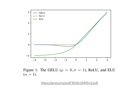
                            model.encoder.layer[0].output.LayerNorm.bias)

output_dense 我们只是通过线性层传递连接的注意力结果。然后我们需要进行归一化，但我们可以看到，我们不是立即对 output_dense 进行归一化，而是首先将其与我们的初始嵌入相加——这称为残差连接。当我们增加神经网络的深度时，即堆叠越来越多的层时，我们会遇到梯度消失/爆炸的问题，当梯度消失的情况下，模型无法再学习，因为传播的梯度接近于零初始层停止改变权重并改进。当权重因极端更新而最终爆炸（趋于无穷大）而无法稳定时，梯度爆炸的相反问题。现在，正确初始化权重和归一化有助于解决这个问题，但观察到的是，即使网络变得更加稳定，性能也会随着优化的困难而下降。添加这些残差连接有助于提高性能，即使我们不断增加深度，网络也变得更容易优化。 out_layernorm 中也使用了残差连接，它实际上是第一个 BertLayer 的输出。最后要注意的是，当我们计算 interterm_dense 时，在将 AttentionLayer 的输出传递到线性层之后，会应用非线性 GeLU 激活函数。 GeLU 表示为：

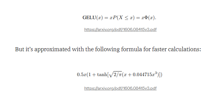
查看图表我们可以看到，如果由公式 max(input, 0) 给出的 ReLU 在正域中是单调的、凸的和线性的，那么 GeLU 在正域中是非单调的、非凸的和非线性的 正域，因此可以逼近更容易复杂的函数。

我们现在已经成功地复制了整个 BertLayer。 该层的输出（与初始嵌入的形状相同）进入下一个 BertLayer，依此类推。 总共有 12 个 BertLayers。 因此，将所有这些放在一起，我们可以从编码器中获得所有 3 个示例的最终结果：

n_batch = 3
tot_n_layers = 12
tot_n_heads = 12
shape_embs = (inputs_tests['input_ids'].shape) + (model.embeddings.word_embeddings.weight.shape[1], )
w_embs_batch = torch.index_select(model.embeddings.word_embeddings.weight, 
                                  0, inputs_tests['input_ids'].reshape(1,-1).squeeze(0)).reshape(shape_embs)
pos_embs_batch = torch.index_select(model.embeddings.position_embeddings.weight, 0, 
                                    torch.tensor(range(inputs_tests['input_ids'][1].size(0))).repeat(1, n_batch).squeeze(0)).reshape(shape_embs)
type_embs_batch = torch.index_select(model.embeddings.token_type_embeddings.weight, 0, 
                                     inputs_tests['token_type_ids'].reshape(1,-1).squeeze(0)).reshape(shape_embs)
batch_all_embs = w_embs_batch + pos_embs_batch + type_embs_batch
normalized_embs = layer_norm(batch_all_embs, model.embeddings.LayerNorm.weight, model.embeddings.LayerNorm.bias)
extended_attention_mask = inputs['attention_mask'].unsqueeze(1).unsqueeze(2)
extended_attention_mask = (1.0 - extended_attention_mask) * -10000.0
for layer_n in range(tot_n_layers):
 if layer_n == 0:
   # compute Q, K and V matrices
   Q = normalized_embs @ model.encoder.layer[layer_n].attention.self.query.weight.T + \ 
                         model.encoder.layer[layer_n].attention.self.query.bias
   K = normalized_embs @ model.encoder.layer[layer_n].attention.self.key.weight.T + \
                         model.encoder.layer[layer_n].attention.self.key.bias
   V = normalized_embs @ model.encoder.layer[layer_n].attention.self.value.weight.T + \
                         model.encoder.layer[layer_n].attention.self.value.bias
   # reshape
   new_x_shape = Q.size()[:-1] + (n_att_heads, att_head_size)
   Q_reshaped = Q.view(*new_x_shape)
   K_reshaped = K.view(*new_x_shape)
   V_reshaped = V.view(*new_x_shape)
   # compute attention probabilities
   att_scores = (Q_reshaped.permute(0, 2, 1, 3) @ K_reshaped.permute(0, 2, 1, 3).transpose(-1, -2))
   att_scores = (att_scores/ math.sqrt(att_head_size)) + extended_attention_mask
   attention_probs = torch.nn.Softmax(dim=-1)(att_scores)
   # concatenate attention heads
   att_heads = []
   for i in range(tot_n_heads):
    att_heads.append(attention_probs[:, i] @ V_reshaped[:, : , i, :])

   output_dense = torch.cat(att_heads, 2) @ model.encoder.layer[layer_n].attention.output.dense.weight.T + \
                                            model.encoder.layer[layer_n].attention.output.dense.bias
   # normalization + residual connection
   output_layernorm = layer_norm(output_dense + normalized_embs, 
                                 model.encoder.layer[layer_n].attention.output.LayerNorm.weight,
                                 model.encoder.layer[layer_n].attention.output.LayerNorm.bias)
   # linear layer + non linear gelu activation
   interm_dense = torch.nn.functional.gelu(output_layernorm @ model.encoder.layer[layer_n].intermediate.dense.weight.T + \
                                           model.encoder.layer[layer_n].intermediate.dense.bias)
   # linear layer
   out_dense = interm_dense @ model.encoder.layer[layer_n].output.dense.weight.T + model.encoder.layer[layer_n].output.dense.bias
   # normalization + residual connection
   out_layernorm = layer_norm(out_dense + output_layernorm, 
                              model.encoder.layer[layer_n].output.LayerNorm.weight, 
                              model.encoder.layer[layer_n].output.LayerNorm.bias)
 else:
   # compute Q, K and V matrices
   Q = out_layernorm @ model.encoder.layer[layer_n].attention.self.query.weight.T + \
                              model.encoder.layer[layer_n].attention.self.query.bias
   K = out_layernorm @ model.encoder.layer[layer_n].attention.self.key.weight.T + \
                              model.encoder.layer[layer_n].attention.self.key.bias
   V = out_layernorm @ model.encoder.layer[layer_n].attention.self.value.weight.T + \
                              model.encoder.layer[layer_n].attention.self.value.bias
   # reshape
   Q_reshaped = Q.view(*new_x_shape)
   K_reshaped = K.view(*new_x_shape)
   V_reshaped = V.view(*new_x_shape)
   # compute attention probabilities
   att_scores = (Q_reshaped.permute(0, 2, 1, 3) @ K_reshaped.permute(0, 2, 1, 3).transpose(-1, -2))
   att_scores = (att_scores/ math.sqrt(att_head_size)) + extended_attention_mask
   attention_probs = torch.nn.Softmax(dim=-1)(att_scores)
   # concatenate attention heads
   att_heads = []
   for i in range(tot_n_heads):
    att_heads.append(attention_probs[:, i] @ V_reshaped[:, : , i, :])

   output_dense = torch.cat(att_heads, 2) @ model.encoder.layer[layer_n].attention.output.dense.weight.T + \
                                            model.encoder.layer[layer_n].attention.output.dense.bias
   # normalization + residual connection
   output_layernorm = layer_norm(output_dense + out_layernorm, 
                                 model.encoder.layer[layer_n].attention.output.LayerNorm.weight, 
                                 model.encoder.layer[layer_n].attention.output.LayerNorm.bias)

   # linear layer + non linear gelu activation
   interm_dense = torch.nn.functional.gelu(output_layernorm @ model.encoder.layer[layer_n].intermediate.dense.weight.T + \
                                                              model.encoder.layer[layer_n].intermediate.dense.bias)
   # linear layer
   out_dense = interm_dense @ model.encoder.layer[layer_n].output.dense.weight.T + model.encoder.layer[layer_n].output.dense.bias
   # normalization + residual connection
   out_layernorm = layer_norm(out_dense + output_layernorm, 
                              model.encoder.layer[layer_n].output.LayerNorm.weight, 
                              model.encoder.layer[layer_n].output.LayerNorm.bias)

注意 out_layernorm – 每层的输出如何被馈送到下一层。
我们可以看到这与 out_view 中的结果相同

 torch.allclose(out_view[-2][-1], out_layernorm, atol=1e-05) # True

Pooler
现在我们可以获取最后一个 BertLayer 的第一个令牌输出，即 [CLS]，将其通过一个线性层并应用一个 Tanh 激活函数来获得池化输出。使用第一个标记进行分类的原因来自于模型是如何被训练为 Bert state 的作者的：
每个序列的第一个标记始终是一个特殊的分类标记 ([CLS])。与该标记对应的最终隐藏状态用作分类任务的聚合序列表示。

 out_pooler = torch.nn.functional.tanh(out_layernorm[:, 0] @ model.pooler.dense.weight.T + model.pooler.dense.bias)

分类器
最后，我们创建一个简单的类，它将是一个简单的线性层，但您可以向它添加一个 dropout 和其他东西。我们在这里假设一个二元分类问题（output_dim=2），但它可以是任何维度的。

from torch import nn
class Classifier(nn.Module):
    
    def __init__(self, output_dim=2):
        super(Classifier, self).__init__()
        self.classifier = nn.Linear(model.config.hidden_size, output_dim, bias=True)
    
    def forward(self, x):
        return self.classifier(x)
classif = Classifier()
classif(out_pooler)
tensor([[-0.2918, -0.5782],
        [ 0.2494, -0.1955],
        [ 0.1814,  0.3971]], grad_fn=<AddmmBackward>)

引用：

 
https://arxiv.org/pdf/1606.08415v3.pdf
https://arxiv.org/pdf/1810.04805.pdf
https://jalammar.github.io/illustrated-transformer/
https://github.com/huggingface/transformers/