介绍

人类有能力理解单词并轻松地从中获取含义。然而，在当今世界，大多数任务都是由计算机执行的。例如，如果您想知道今天是晴天还是下雨天，则必须在 Google 中输入文本查询。现在的问题是，机器将如何频繁地理解和处理文本中呈现的如此大量的信息？答案是词嵌入。

Word Embeddings 基本上是向量（文本转换为数字），用于捕获单词的含义、各种上下文和语义关系。嵌入本质上是使用预定义字典将单词映射到其对应向量。

例如，

句子： It will rain heavily today.

字典：{“it”：[1,0,0,0,0]，“will”：[0,1,0,0,0]，“rain”：[0,0,1,0,0] , “ heavily ”: [0,0,0,1,0], “today”: [0,0,0,0,1]}

在这里，每个单词都被分配了一个唯一的向量（例如），以便区分所有单词。

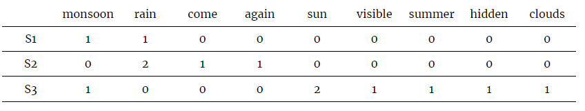
Let the corpus comprise three sentences.

S1 = In monsoon, it will rain.

S2 = rain rain come again.

S3 = sun is visible in summer. In the monsoon, the sun is hidden by clouds.

Let N be the list of unique words = [‘monsoon’, ‘rain’, ‘come’, ‘again’, ‘sun’, ‘visible’, ‘summer’, ‘hidden’, ‘clouds’]

计数矩阵的维度将是 3X9，因为语料库中有 3 个文档和 9 个唯一词。
计数矩阵如下所示：

优点：由于只考虑单词的频率，因此计算成本较低。

缺点：由于计算只是基于计数并且没有考虑单词的上下文，因此该方法证明不太有用。
代码：

#Importing libraries
from sklearn.feature_extraction.text import CountVectorizer
import nltk 
from nltk.corpus import stopwords 
from nltk.tokenize import word_tokenize 

#Downloading stopwords and punkt packages
nltk.download('stopwords') 
nltk.download('punkt') 

#Initialising stopwords for english
set(stopwords.words('english')) 

#sample sentences
text = ["In monsoon, it will rain", "rain rain come again", "sun is visible in summer. In the monsoon, the sun is hidden by clouds"]

#set of stop words
stop_words = set(stopwords.words('english')) 
all_sentences = []

#Logic for removing stop words and obtaining filtered sentences from the list 

for i in range(len(text)):
  word_tokens[i] = word_tokenize(text[i]) 
  tokenized_sentence = []

  for j in word_tokens[i]: 
      if j not in stop_words: 
          tokenized_sentence.append(j) 
  all_sentences.append(" ".join(tokenized_sentence))

#Initialising the CountVectorizer
countvectorizer = CountVectorizer()

#Applying CountVectorizer to the list of sentences
X = countvectorizer.fit_transform(all_sentences)

#Converting output to array
result = X.toarray()

print("Sentences after removing stop words", all_sentences)
print("Count Vector:", result)

2.TF-IDF：

TF-IDF 代表词频-逆文档频率。 该方法是对 Count Vector 方法的即兴创作，因为特定单词的频率被考虑在整个语料库中，而不仅仅是单个文档。 主要思想是对某些文档非常具体的词给予更多的权重，而对更普遍且在大多数文档中出现的词给予较少的权重。

例如，诸如“is”、“the”、“and”之类的通用词会经常出现，而诸如“Donald Trump”或“Indira Gandhi”之类的词将特定于特定文档。

数学上，

词频 (TF) = 词条在文档中出现的次数 / 文档中词条的总数

逆文档频率 (IDF) = log(N/n) 其中 N 是文档总数，n 是一个术语出现的文档数。

考虑以下示例。
给出了两个文档——D1 和 D2。

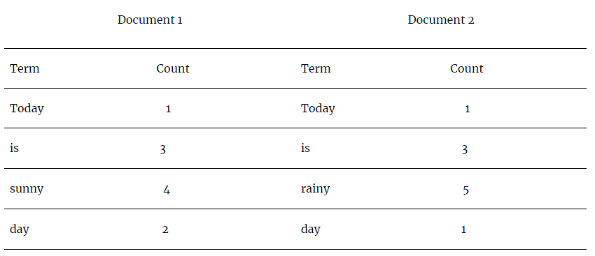
TF(Today, Document 1) = 1/8

TF(Today, Document 2) = 1/8

TF(sunny, Document 1) = 4/8

IDF(Today) = log(2/2) = log(1) = 0

IDF(sunny) = log(2/1) = log(2) = 0.301

Therefore,

TF-IDF(Today, Document 1) = 1/8 * 0 = 0

TF-IDF(Today, Document 2) = 1/8 * 0 = 0

TF-IDF(sunny, Document 1) = 4/8 * 0.301 = 0.1505

从上面的计算可以看出，与文档 1 的上下文中的重要词“sunny”相比，常用词“Today”的权重较低。

优点：

它在计算上很容易。
文档中最重要的单词是通过基本计算提取的，不需要太多努力。

缺点：

它无法捕捉单词的语义，只能像词汇级别的特征一样工作。
代码：

from sklearn.feature_extraction.text import TfidfVectorizer 
import pandas as pd

#Declaring the list of sentences
documents = ['Today is sunny day', 'Today is rainy day']

#Initialising Tfidf Vectorizer
vectorizer = TfidfVectorizer()

#Fitting the Vectorizer to the list
X = vectorizer.fit_transform(documents)
print(X)

#Printing the feature names
print(vectorizer.get_feature_names()) 

matrix = X.todense()
tfidf_list = matrix.tolist()
tfidf_df = pd.DataFrame(tfidf_list, columns = vectorizer.get_feature_names())

print(tfidf_df)

3.Word2Vec：

Word2Vec 是一种基于预测的词嵌入方法。 与确定性方法不同，它是一个浅层的两层神经网络，能够预测单词之间的语义和相似性。 Word2Vec 是两种不同模型的组合——（i）CBOW（连续词袋）和（ii）Skip-gram。

模型概述 – CBOW（连续词袋）和 Skip-gram。

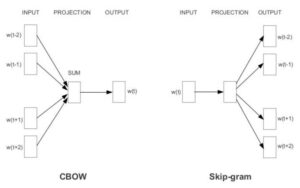
3.1 CBOW（连续词袋）：

该模型是一个浅层神经网络，可以在给定上下文的情况下预测单词的概率。 这里，上下文是指围绕要预测的单词的单词的输入。
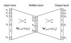
CBOW模型的架构：

作为第一步，输入是通过为给定文本形成一个词袋来创建的。
例如，

Sentence 1 = All work and no play make Jack a dull boy.

Sentence 2 = Jack and Jill went up the hill.

Bag of Words: {“All”:1, “work”:1, “no”:1, “play”:1, “makes”:1, “Jack”:2, “dull”:1, “boy”:1, “Jill”:1, “went”:1, “up”:1, “hill”:1} (after removing the stop words)

这个由单词及其出现频率组成的输入作为向量发送到输入层。对于 X 个单词，输入将是 X[1XV] 个向量，其中 V 是向量的最大长度。

接下来，输入隐藏层矩阵由维数 VXN 组成，其中 N 是表示单词的维数。输出隐藏层矩阵由维数 NXV 组成。在这里，这些值是通过将输入乘以隐藏输入权重来计算的。

在输出层，通过将隐藏输入乘以隐藏输出权重来计算输出。在隐藏层和输出层之间计算的权重给出了单词的表示。作为一个连续的中间步骤，通过对输出和目标值之间计算的误差使用反向传播来调整权重。
优点：

与确定性方法相比，概率性方法给出了更好的结果。
由于不需要计算巨大的矩阵，因此内存需求较少。
缺点：

优化非常重要，否则培训将需要很长时间才能完成。

3.2 Skip-gram ：

Skip-gram 模型预测给定单词的上下文，与 CBOW 所做的正好相反。 Skip-gram 模型的架构：

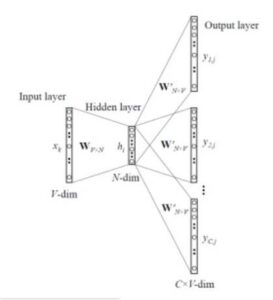
输入层大小：[1XV]，输入隐藏权重矩阵大小：[VXN]，输出隐藏权重矩阵：[NXV]，输出层大小：C[1XV]

模型的输入和直到隐藏层的进一步步骤将类似于 CBOW。 输出目标变量的数量取决于上下文窗口的大小。 例如，如果上下文窗口的大小为 2，那么将有四个目标变量，两个词在给定词之前，两个词在给定词之后。

将针对四个目标变量计算四个单独的误差，并通过执行元素相加获得最终向量。 然后反向传播这个最终向量以更新权重。 对于训练，输入和隐藏层之间的权重用于单词表示。

优点：

Skip-gram 模型可以捕获单词的不同上下文信息，因为每个上下文都有不同的向量表示。
对于不常用的术语更准确，并且适用于更大的数据库。
缺点：

它需要更多的 内存 进行处理。
代码：

要使用 genism 库中预训练的 Word2Vec 模型：

import gensim 
import gensim.downloader as api
from gensim.models.keyedvectors import KeyedVectors

#loading pretrained model
nlp_w2v = api.load("word2vec-google-news-300") 

#save the Word2Vec model
nlp_w2v.wv.save_word2vec_format('model.bin', binary=True)

#load the Word2Vec model 
model = KeyedVectors.load_word2vec_format('model.bin', binary=True)

#Printing the most similar words to New York from vocabulary of pretrained model
model.most_similar('New_York')

从头开始训练 Word2Vec 模型：

import gensim 
'''
Data for training Word2Vec
train: A data frame comprising of text samples
'''

#training data
corpus = train

#creates a list for a list of words for every training sample
w2v_corpus = []
for document in corpus:
   w2v_words = document.split()
   w2v_grams = [" ".join(w2v_words[i:i+1]) 
               for i in range(0, len(w2v_words), 1)]
   w2v_corpus.append(w2v_grams)

#initialising and training the custom Word2Vec model 
'''
size: dimensions of word embeddings 
window: context window for words 
min_count: words which appear less number of times than this count will be ignored 
sg: To choose skip-gram model 
iter: Number of epochs for training
'''

word2vec_model = gensim.models.word2vec.Word2Vec(w2v_corpus, size=300,   
            window=8, min_count=1, sg=1, iter=30)

#vector size of the model
print(word2vec_model.vector_size)

#vocabulary contained by the model
print(len(word2vec_model.wv.vocab))

4.GloVE:

GloVe 代表词表示的全局向量。 该算法是对 Word2Vec 方法的改进，因为它考虑全局统计而不是局部统计。 在这里，全局统计数据意味着从整个语料库中考虑的单词。 GloVe 基本上试图解释特定单词对在文档中出现的频率。 为此，构建了一个共现矩阵，该矩阵将表示特定单词相对于另一个单词的存在。

例如，

Corpus – It is rainy today, tomorrow it will be sunny and the day after will be windy.

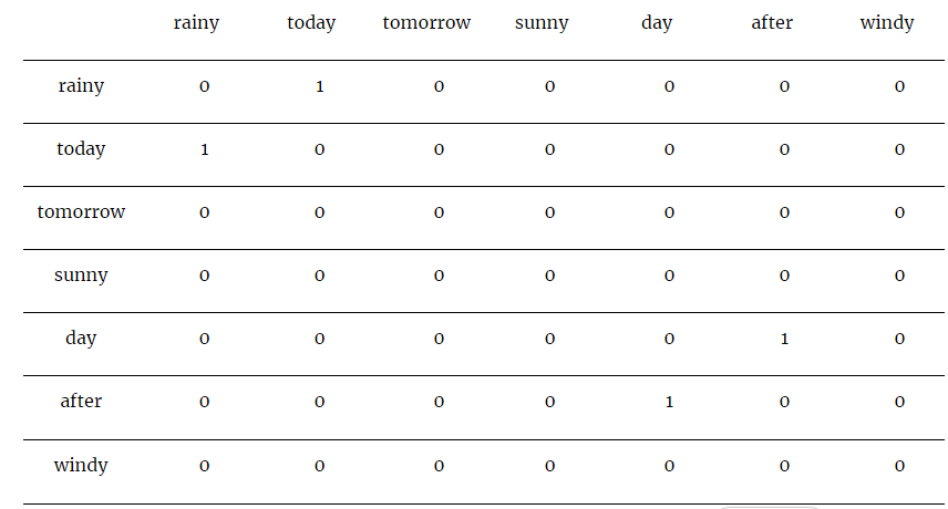
上面的矩阵表示一个共现矩阵，其值表示在给定示例语料库中一起出现的每对单词的计数。

在计算给定“today”、p(rainy/today) 和给定“tomorrow”、p(rainy/tomorrow) 的单词“rainy”的出现概率后，结果是与“rainy”最相关的单词 与“明天”相比，“今天”是“今天”。

代码：

#Import statements
from numpy import array
from numpy import asarray
from numpy import zeros
from keras.preprocessing.text import Tokenizer 

#Download the pretrained GloVe data files
!wget http://nlp.stanford.edu/data/glove.6B.zip

#Unzipping the zipped folder
!unzip glove*.zip

#Initialising a tokenizer and fitting it on the training dataset
'''
train: a dataframe comprising of rows containing text data
'''
tokenizer = Tokenizer(num_words=5000)
tokenizer.fit_on_texts(train)

#Creating a dictionary to store the embeddings
embeddings_dictionary = dict()

#Opening GloVe file
glove_file = open('glove.6B.50d.txt', encoding="utf8")

#Filling the dictionary of embeddings by reading data from the GloVe file
for line in glove_file:
    records = line.split()
    word = records[0]
    vector_dimensions = asarray(records[1:], dtype='float32')
    embeddings_dictionary[word] = vector_dimensions
glove_file.close()

#Parsing through all the words in the input dataset and fetching their corresponding vectors from the dictionary and storing them in a matrix 
embedding_matrix = zeros((vocab_size, 50))
for word, index in tokenizer.word_index.items():
    embedding_vector = embeddings_dictionary.get(word)
    if embedding_vector is not None:
        embedding_matrix[index] = embedding_vector

#Displaying embedding matrix 
print(embedding_matrix) 

结论：

在这篇博客中，我们回顾了一些方法——Count Vector、TF-IDF、Word2Vec 和 GloVe，用于从原始文本数据创建词嵌入。 预处理文本然后发送预处理数据以创建词嵌入总是一个好习惯。 作为进一步的步骤，这些词嵌入可以发送到机器学习或深度学习模型，用于各种任务，例如文本分类或机器翻译。